Let's say that we have the following system:

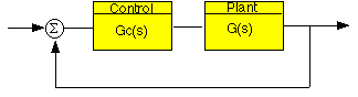
We can view the open loop Bode plot of this system by looking at the Bode plot of Gc(s)G(s). However, we can also view the Bode plots of G(s) and of Gc(s) and add them graphically. Therefore, if we know the frequency response of simple functions, we can use them to our advantage when we are designing a controller:

	bode(1, [1 0])

1
---
s

	bode(1, [1 1])

1
------
s + 1

	bode([1 0], 1)

s

	bode([1 1], 1)

s+1

Note that the location of the pole or zero(a) will greatly affect the frequency response. If we have a pole close to the origin, the response at lower frequencies will undergo the most drastic changes. If we have a pole or zero farther from the origin, the response at higher frequencies will undergo the most drastic changes. Also remember that a change in gain will shift the entire gain response up or down and will not affect the phase. Let's see a couple of examples:

	bode(1,[ 1, 0.1])

1
------
s + 0.1

	bode(1,[ 1, 10])

1
------
s + 10

	bode([1, 0.1],1)

s + 0.1

	bode([1, 10],1)

s + 10

Modifying the location of these poles or zeros, we can manipulate the frequency response of the combined system to something that will suit our purposes.

Use your browser's "Back" button to return to the previous page

8/27/96 LJO